Discrete Differential Geometry and Graph Convolution
TL;DR
The graph laplacian is the same laplacian operator in terms of discrete differential geometry.
Convolution can be defined in terms of Fourier transform.
Fourier transform can be defined in terms of eigenfunctions of laplacian operator.
Therefore, we can define graph convolution by the graph laplacian.
Geometric Deep Learning and Graph Neural Network
Deep Learning is one of the most greatest advance in machine learning. But, mathematically, neural network is just a parameterized function $\renewcommand{\R}{\mathbb{R}}f_{\theta}: \mathbb{R}^n \rightarrow \mathbb{R}^m$ and there is no way to enforce geometric structure of its domain to neural network.
For example, let us assume that our domain is graph $\mathcal{G} = (\mathcal{V}, \mathcal{E})$. Typically in graph machine learning, there is a node feature vector $X_v \in \mathbb{R}^d$ for each $v \in \mathcal{V}$.
Then we can make a neural network which gets input $X = \left[X_{v_1}, X_{v_2}, \cdots, X_{v_{|\mathcal{V}|}}\right] \in \mathbb{R}^{|\mathcal{V}| \times d}$, and adjacency matrix $A$.
Since the ordering of graph does not have meaning,
\[f_{\theta} \left(X_{v_{\sigma(1)}}, \cdots, X_{v_{\sigma(|\mathcal{V}|)}}, PAP^T\right) = f_{\theta} \left(X_{v_1}, \cdots, X_{v_{|\mathcal{V}|}}, A\right)\]should hold for every permutation $\sigma$ and corresponding permutation matrix $P$ (this property is called permuation invariance), or
\[f_{\theta} \left(X_{v_{\sigma(1)}}, \cdots, X_{v_{\sigma(|\mathcal{V}|)}}, PAP^T\right) = Pf_{\theta} \left(X_{v_1}, \cdots, X_{v_{|\mathcal{V}|}}, A\right)\]should hold(this property is called permutation equivariance).
But there is no way to enforce these structures to $f_{\theta}$.
Geometric Deep Learning is a research field of deep learning, which studies to construct neural network with geometric ‘symmetry’ of domain. The major domains of geometric deep learning is Grids, Groups, Graphs, Geodesics, and Gauges.
Ordinary convolutional layer is a well-known instance of geometric deep learning. It is ‘equivariant’ layer of ‘Grid’.
For ‘Graph’, we want to make a permutation equivariant layer with the ordering of graph. The discrete differential geometry can propose an answer to this question, which we call (spectral) graph convolution.
Prerequisite: Differential Geometry
Riemannian Manifold
Definition (Riemannian Manifold).
A Riemannian manifold $M$ is a smooth manifold equipped smooth $(0,2)$-tensor field(bilinear form) $\renewcommand{\R}{\mathbb{R}}g_p : T_p M \times T_p M \rightarrow \R$ such that
\[\begin{align} &g_p(X, Y) = g_p(Y, X) & \textrm{(Symmetric)} \\ &&\\ &g_p(X, X) \geq 0 \textrm{ and } g_p(X,X) = 0 \Longleftrightarrow X = 0 & \textrm{(Positive definite)} \end{align}\]$g_p$ is called a Riemannian metric. In fact, it is a smooth assignment of inner product for each $T_p M$.
Therefore, we also write $g_p(X,Y)=\left<X, Y\right>_p$
With the Riemannian metric, we can define a ‘orthonormal’ frame.
Definition (Riemannian Orthonormal Frame).
A Riemannian Orthonormal Frame is a local frame which satisfies
\[\newcommand{\ip}[1]{\left< #1 \right>} g_p (X_i(p), X_j(p)) = \ip{X_i(p), X_j(p)} = \delta_{ij}\]Volume Form
Orientation via differential form
We have seen that
\[d\tilde{x}_1 \wedge \cdots \wedge d\tilde{x}_n = \det \left(\frac{\partial \tilde{x}_j}{\partial x_i}\right) dx_1 \wedge \cdots \wedge dx_n\]holds for two local coordinate system $(x_1,\cdots, x_n), \; (\tilde{x}_1, \cdots, \tilde{x}_n)$.
Therefore, we can also define orientability in terms of differential form.
Theorem (Orientation via nonvanishing $n$-form).
$M$ is orientable if and only if there exists a $n$-form $\omega$ such that $\omega \neq 0$ everywhere.
Volume Form
Definition (Volume Form).
A volume form is a $n$-form on $n$-manifold $M$ is a nonvanishing form. we write volume form as $\textrm{vol}_n$, or $dV$.
Existence of the volume form is equivalent to orientability.
For Riemannian manifold, due to the Riemannian metric, we can define a ‘natural’ volume form.
Definition (Riemannian Volume Form).
A Riemannian volume form is a $n$-form such that $\omega(E_1, \cdots, E_n) = 1$ for every orthonormal frame $E=(E_1,\cdots, E_n)$.
Let $\varepsilon_i$ be a coframe(dual) of $E_i$, then we can write
\[\textrm{vol}_n = \varepsilon_1 \wedge \cdots \wedge \varepsilon_n\]Proposition.
For a local coordinate system $(U, x)$,
\[\textrm{vol}_n = \sqrt{|\det (g_{ij})|} dx_{1}\wedge \cdots \wedge dx_n\]where $g_{ij}$ is local coordinate representation of the Riemannian metric.
proof.
Let us represent local coordinate basis as orthonormal frame.
\[\frac{\partial}{\partial x_i} = \sum_{j} A_{ij} E_j\]Then,
\[\newcommand{\pdiv}[1]{\frac{\partial}{\partial x_{#1}}} g_{ij} = \ip{\pdiv{i}, \pdiv{j}}_p = \sum_{k, l} A_{ik}A_{jl} \ip{E_k, E_j}_p =\sum_{k} A_{ik}A_{jk} = (AA^T)_{ij}\]Then,
\[\newcommand{\vol}{\textrm{vol}} \vol_n \left(\pdiv{1},\cdots, \pdiv{n}\right) = \varepsilon_1 \wedge \cdots \wedge \varepsilon_n \left(\pdiv{1}, \cdots, \pdiv{n}\right) = \det(A_{ij})\]Finally, $\det (g_{ij}) = \det(AA^T) = (\det A)^2$
Therefore,
\[\vol_n = \det A dx_1 \wedge \cdots \wedge dx_n = \sqrt{|\det(g_{ij})|} dx_1 \wedge \cdots \wedge dx_n\]Remark
In $\R^n$, volume form is just a $\det$. Note that when we have linearly independent vectors $v_1, \cdots, v_n$, then the volume of parallelepiped generated by $v_1,\cdots, v_n$ is $\det(v_1,\cdots, v_n)$.
Let $X = (X_1(u, v), X_2(u, v), X_3(u, v))$ be a parametrized surface. Then the volume form $dS = |X_u \times X_v| dudv$ is the area element in surface integral.
Hodge Star
Definition (Hodge Star).
Since we represented $k$-form as
\[\omega = \sum_{i_1 < \cdots < i_{k}} \omega_{i_1, \cdots, i_k} dx_{i_1} \wedge \cdots \wedge dx_{i_k} \in \Lambda^{k}(V)\]$\dim \Lambda^{k}(V) = \binom{n}{k} = \binom{n}{n-k} = \dim\Lambda^{n-k}(V) $.
Therefore, we can define a natural isomorphism $\star:\Lambda^{k}(V)\rightarrow\Lambda^{n-k}(V)$.
\[\star(dx_{i_1} \wedge \cdots dx_{i_k}) = dx_{j_1} \wedge \cdots \wedge dx_{j_{n-k}}\]where $(i_1,\cdots, i_k, j_1, \cdots, j_{n-k})$ is a even permutation of $(1, \cdots, n)$.
Moreover, let $M$ be a Riemannian manifold, Let $\varepsilon_{i}$ be a orthonormal coframe, then
\[\star(\varepsilon_{i_1} \wedge \cdots \varepsilon_{i_k}) = \varepsilon_{j_1} \wedge \cdots \wedge \varepsilon_{j_{n-k}}\]where $(i_1,\cdots, i_k, j_1, \cdots, j_{n-k})$ is a even permutation of $(1, \cdots, n)$.
The Riemannian volume form can be expressed by a hodge star, $\vol_n=\star (1)$, where the 1 is $f: M \rightarrow \R$ such that $f(p) = 1$ everywhere.
Definition (Inner Product by Hodge Star).
Let $\alpha, \beta$ be a $k$-form, then we can define an inner product by
\[\newcommand{\iip}[1]{\left<\left< #1 \right>\right>} \iip{\alpha, \beta} = \int_{M} \alpha \wedge\star\beta = \ip{\alpha, \beta}_g \int_{M} \vol_n = \ip{\alpha, \beta}_g \vol_n (M)\]where $\ip{\cdot, \cdot}_g$ is $\ip{\alpha_1\wedge \cdots \wedge \alpha_k, \beta_1\wedge\cdots\beta_k}_g = \det(\ip{\alpha_i, \beta_j})$.
Properties of Hodge Star
- $\star\star \omega = (-1)^{k(n-k)}\omega$
Remark
- Generally, hodge star is defined by the equation $\alpha \wedge \star \beta = \ip{\alpha, \beta}_g\vol_n $.
Codifferential
Definition (Codifferential).
Codifferential is an operator maps $k$-form to $(k-1)$-form by
\[\delta = (-1)^{k} \star^{-1} d \star\]Note that two stars between $d$ has different dimension.
Remark
- Codifferential and exterior derivative are adjoint with respect to hodge star inner product, $\iip{d\alpha, \beta} = \iip{\alpha, \delta\beta}$
Laplacian
For $f: \R^n \rightarrow \R$, we defined laplacian operator
\[\Delta f = \sum_{i=1}^{n} \frac{\partial^2 f}{\partial x_i^2}\]Now we can generalize this operator to any $k$-form on manifold, which called Laplace-Beltrami operator or Laplace-de Rham operator.
Definition (Laplace-Beltrami Operator, Laplace-de Rham Operator).
\[\Delta_k = \delta d + d\delta\]
Remark
When $k=0$ and $M=\R^n$, then $d\delta=0$ and
\[\begin{align*} \Delta_0 f &=\delta d f =\star^{-1} d \star d f \\ &= \star d \star df = (\star d \star) \left(\sum_{i=1}^{n}\frac{\partial f}{\partial x_i} dx_i\right)\\ &= \star d \left(\sum_{i=1}^{n}\frac{\partial f}{\partial x_i} (-1)^{i} dx_1 \wedge \cdots \wedge d\hat{x}_i \wedge \cdots \wedge dx_n\right) \\ &= \star \left(\sum_{i=1}^{n} \frac{\partial^2 f}{\partial x_i^2} dx_1 \wedge \cdots \wedge dx_n \right)\\ &= \sum_{i=1}^{n} \frac{\partial^2 f}{\partial x_i^2} \end{align*}\]is the ordinary laplacian.
Some authors may define the sign of laplacian differently.
Prerequisite: Algebraic Topology
You may skip the sections about homology and cohomology if you are not interested in.
Simplicial Complex
Simplicial complex is a way to represent topological space by vertices.
Simplex
Let $\renewcommand{\R}{\mathbb{R}}v_0,\cdots, v_p \in \R^p$ such that $v_1 - v_0, \cdots, v_p - v_0$ are linearly independent.
Definition (Geometric Simplex).
A geometric $p$-simplex $\sigma_p = [v_0,\cdots, v_p]$ is a convex hull of $v_0,\cdots, v_{p}$, i.e.
\[ [v_0, v_1, \cdots, v_p] = \left\{ \sum_{i=0}^{p} t_i v_i : 0\leq t_i \leq 1, \; \sum_{i=0}^{p} t_i = 1 \right\}\]and each $v_i$ is called a vertex of simplex.
The standard $p$-simplex is
\[\Delta^p = [e_0,\cdots, e_p] \subset \R^p, e_0 = (0,\cdots, 0)\]We define a simplex spanned by a nonempty subset of vertices of $\sigma_p$ is a face of $\sigma_p$. i.e. $[v_{i_0}, \cdots, v_{i_k}]$ for some $1 \leq i_0<\cdots< i_k \leq p$ .
and we define $i$th boundary face $F_{i,p}=[v_0,\cdots, \hat{v}_i,\cdots, v_p]$. ($\hat{v}_i$ means $v_i$ is omitted)
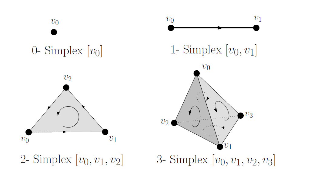 Image from: Muhammad, A and Magnus, E. 2006
Simplicial Complex
Simplicial complex is the collections of simplicies together represents a topological space.
Definition (Simplicial Complex).
A simplicial complex $K$ is a collection of simplicies of various dimensions satisfying
- If $\sigma \in K$, then every face of $\sigma$ is in $K$
- The intersection of any two simplicies in $K$ is either empty or a face of each.
We denote a collection of all $p$-simplicies in $K$ by $K_p$.
 Image from: wikipedia
Chain Group
Definition (Chain Group).
Let $K_p$ be a $p$-simplex contained in simplical complex $K$, then we define a chain group $C_p(K)$ by
\[C_p(K)=\{ c_1 \sigma_1 + \cdots + c_{|K_p|} \sigma_{|K_p|}: c_i \in \mathbb{Z}\} = \left < \sigma_1, \cdots, \sigma_{|K_p|} \right> \simeq \mathbb{Z}^{|K_p|}\], where the sum and multiplication is just a formal sum and formal multiplication.
With the multiplication and sum operation on chain, we can define orientation by
\[(v_{\sigma(0)}, \cdots, v_{\sigma(p)})=\textrm{sgn}(\sigma)[v_0,\cdots, v_p]\]for any permutation $\sigma$.
Boundary
Definition (Boundary).
We can define the boundary map $\partial_i: C_p (K) \rightarrow C_{p-1}(K)$ by
\[\partial_i [v_0, \cdots, v_p] = \sum_{i} (-1)^{i} F_{i, p}\]Note that the boundary map is a group homomorphism from $C_p(K)$ to $C_{p-1}(K)$.
The $(-1)^{i}$ factor is to make the boundary counter-clockwise.
Below image is helpful to understand the intution behind chain group and boundary.
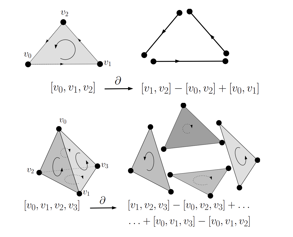 Image from: Muhammad, A and Magnus, E. 2006
Singular Chain
Definition (Singular Simplex).
A $p$-singular simplex in $M$ is a smooth map $\sigma: \Delta^{p} \rightarrow M$.
Definition (Singular Chain).
Similary, a $p$-singular chain is defined by $c=c_1 \sigma_1 + \cdots, + c_k \sigma_k$, where $\sigma_i$ are singular simplex. And we denote the free abelian group $\left< \sigma_1, \cdots, \sigma_k \right> = C_p(M)$ as we did previously.
Definition (Boundary Map).
Let $\sigma$ be a $p$-singular simplex, then the boundary map $\partial_p: C_p(M) \rightarrow C_{p-1}(M) $ is
\[\partial_p \sigma = \sum_{i} (-1)^{i} \sigma \circ F_{i, p}\]and for singular chain $c = \sum_{i} c_i \sigma_i $, then $\partial_p c := \sum_{i} c_i \partial_p \sigma_i$
Chain Complex
Definition (Chain Complex).
Chain complex $C$ is a collcection of pairs \(\{(C_i, \partial_i)\}_{i\in\mathbb{Z}}\) such that $C_i$ are free abelian group and $\partial_i: C_i \rightarrow C_{i-1}$ is a group homomorphism such that \(\partial _i \circ \partial_{i+1}=0\) for all $i$.
We can think chain complex is an algebraic generalization of the notion of complex which we discussed above.
Homology
Definition (Homology).
For a given chain complex $C$, $k$th homology group $H_k$ is
\[H_k(C) = \ker \partial_i/\textrm{im} \partial_{i+1}\]Since $\partial_{i} \circ \partial_{i+1}=0, \textrm{im}\partial_{i+1} \leq \ker \partial_i$ and homology groups are well-defined.
In topology, we consider a space $X$ and given chain complex ${(C_i, \partial_i)}_{i}$, and the chain groups $C_i$ are typically a module over $R$, then we write $H_k(X,R)$
Cohomology
Definition (Cohomology).
Let us given a chain complex \(C = \{(C_i, \partial_i)\}\). Then we have a dual of chain group, called cochain group \(C_n^*=\textrm{Hom}(C_k, G)\) and coboundary map $\delta_k: C_{k-1}^* \rightarrow C_{k}^*$. Then the quotient group
\[H^{k}(C) = \ker \delta_k / \textrm{im } \delta_{k-1}\]is the cohomology group.
de Rham cohomology
Definition (de Rham Cohomology).
Since $d \circ d = 0$, differential forms with the exterior derivative naturally define a cochain complex. The cohomology group of cochain complex of differential forms is the de Rham cohomology
\[H_{DR}^{k}(M) = \ker d_{k} / \textrm{im } d_{k-1}\]Theorem (de Rham).
Let $M$ be a smooth, orientable manifold. $H_{sing}^k(M)$ be a cohomology group given by the singular chain. Then
\[H^{k}_{DR}(M) \simeq H^{k}_{sing}(M, \R)\]Informally speaking, this theorem tells us that the exterior derivative $d$ and the adjoint of the boundary operator $\partial$ has a close relationship.
Recall that someone may write the stokes’ theorem by $\left<\left<M|d\omega\right>\right>=\left<\left<\partial M|\omega\right>\right>$
Discrete Differential Geometry
Now we will define differential forms in discrete space.
Abstract Simplicial Complex
In geometric simplex, we represented simplex as a convex hull in euclidean space.
Now, we will represent it by combinatorial way.
That is, we will represent the space with vertices and their relationship.
First, graph is 1-dimensional simplex, graph represent the space by vertices and its edges, 1-dimensional relationship.
Definition (Abstract Simplicial Complex).
Let \(\mathcal{V}=\{v_0, \cdots, v_n\}\) be a vertex set.
Abstract simplicial complex $K$ is a $K \subset \mathcal{P}(V)$ such that
- $\emptyset \in K$
- $v \in \mathcal{V} \implies \{v\} \in K$
- $X \in K, Y \subset X \implies Y \in K$
As you can see below image, abstract simplicial complex is a discretization of continuous space.
Each $\sigma \in K$ is called a simplex. All other definitions(face, chain group, boundary, …) are same with that of geometric simplex.
 Image from: wikipedia
Discrete Exterior Calculs
First, let us define a differential form.
Definition (Discrete Differential Form).
Let $C_k(K)$ be a chain group. In discrete differential geometry, we can think everything as a vector space.
Therefore, $C^{k}(K)$ is just a dual space such that $f \in C^{k}(K)$ is a linear functional $f: C_k(K)\rightarrow \R$. The $0$-form is a function $f: \mathcal{V} \rightarrow \R$.
Let $v=[v_{i_0}, \cdots, v_{i_k}] \in K_p$, $\omega \in C^{p}(K)$. We can think $v$ as a standard basis of $C_p(K)$. and since $\omega$ is linear,
\[\omega([v_{i_{\sigma(0)}},\cdots, v_{i_{\sigma(p)}}]) = \textrm{sgn }(\sigma) \omega([v_0, \cdots, v_p])\]Thus it naturally satisfies the alternating property.
Intuitively, 0-form is a function on vertex, 1-form is a function on edge, 2-form is a function on face and it extends linearly.
We will also write $\omega(\sigma) = \ip{\omega, \sigma} := \int_{\sigma} \omega$.
It is natural to write it as inner product because the basis and dual basis naturall defines inner product with its coordinate representation. And write it as integral is also natural because each vertex, edge, face, … is a discretization of continuous space. Integral of whole space discretized by sum of function values of each discretized component.
Definition (Discrete Exterior Derivative).
The exterior derivative $d$ is defined to satisfy the stokes’ theorem. i.e.
Let $\omega$ be a $k$-form, then $d\omega$ is the $(k+1)$-form which satisfies
\[\int_{\sigma} d\omega = \int_{\partial \sigma} \omega\]for all $\sigma \in C_{k+1}(K)$.
Examples
1. Let $f$ be a $0$-form, then \(df(v_1, v_2) = \int_{(v_1, v_2)} df = \int_{v_2 - v_1} f = f(v_2) - f(v_1)\)
2. \(\sigma = [v_0, v_1] + \cdots + [v_{n-1}, v_n]\) be a path. Then \(\int_{\sigma} df = \int_{\partial \sigma} f = (f(v_n) - f(v_{n-1})) + \cdots + (f(v_1) - f(v_0))\)
3. \(dw(v_1, v_2, v_3) = \int_{(v_1, v_2, v_3)} dw = \int_{(v_2, v_3)} w - \int_{(v_1, v_3)} w + \int_{(v_1, v_2)} w = w (v_2, v_3) - w(v_1, v_3) + w(v_1, v_2)\)
4. \(w(\partial_{k+1}\sigma)= d_k w (\sigma) = \ip{d_k w, \sigma} = \ip{w, d_k^T \sigma} = w(d_k^T\sigma) \implies d_k^T = \partial_{k+1}\) in matrix representation.
Combinatorial Laplacian
Definition (Graph Laplacian).
Let $D$ be a degree matrix, $A$ be an adjacency matrix of $G$. then the graph laplacian is
\[L := D - A\]Theorem.
Let $\partial_1$ be a matrix representation of boundary map from edge to node. (It is called incidence matrix)
Then
\[L = \partial_1 \partial_1^T\]Definition (Combinatorial Laplacian).
A combinatorial laplacian is the Laplace-de Rham operator in the context of discrete differential geometry.
Let us recall that the codifferential has an adjoint relationship
\[\iip{d\alpha, \beta} = \iip{\alpha, \delta \beta}\]First, note that I treated abstract simplicial complex just a combinatorial generalization of graph. But in some other materials, we can give a notion of volume on each simplex.
In this context, I’ll set $\vol(K) =1$.
And, since we defined $\alpha(\sigma) = \int_{\sigma} \alpha$, in matrix representation, $\delta = d^{T}$.
thus, a combinatorial laplacian is defined by
\[\Delta_k = d_k^T d_k + d_{k-1} d_{k-1}^T\]Furthermore, since $d_k^T = \partial_{k+1}$, we also write
\[\Delta_k = \partial_{k+1} \partial_{k+1}^T + \partial_{k}^T \partial_{k}\]Note that if we define volume for each simplex, then there should be a volume correction factor in hodge star, see (Chern, 2020).
If $k=0$, by the above theorem, we can check the graph laplacian is the same laplacian operator in the context of discrete differential geometry.
Properties of Graph Laplacian
- $L= L^T$
- Row sum and column sum of $L$ is $0$.
- $ (Lv)_i = \sum_{j} A_{ij} (v_i - v_j) = \sum_{(i,j)\in E} (v_i - v_j)$
- $v^T L v = \sum_{(i,j) \in E} (v_i - v_j)^2 \implies L \succeq 0$
Note that since $df = \sum_{i=1}^{n} \frac{\partial f}{\partial x_i} dx_i = \nabla f \cdot (dx_1, \cdots, dx_n)$, in discrete differential geometry, $\nabla f(v_i) = (v_j - v_i)_{(i,j)\in E} \in \R^{|E|}$, the last equality becomes
\[\ip{\Delta v, v} = \ip{\nabla v, \nabla v}\]Graph Convolutional Network(GCN)
Now it’s time to talk about Graph Convolution.
First, we can think node feature vectors
\[X = \left[X_{v_1}, X_{v_2}, \cdots, X_{v_{|\mathcal{V}|}}\right] \in \mathbb{R}^{|\mathcal{V}| \times d}\]is stack of $d$ functions defined on $\mathcal{V}$.
That is, to think $(X_{v_i})_j = f_j(v_i)$, for each $f_j: \mathcal{V} \rightarrow \R \simeq \R^{|\mathcal{V}|}$
Then, it is sufficient to define a convolution operator to each $f_j$, because we can stack multiple convolutional layer to process each channel of input, like convolutional layer for image.
Convolution
Let $\mathcal{F}$ be a fourier trasnform operator, and $ \star $ be a convolution operator. Then
\[\mathcal{F}(f \star g) = \mathcal{F}(f) \mathcal{F}(g)\]holds. With this relationship, let $f, g \in \R^{|\mathcal{V}|} $ be functions defined on $\mathcal{V}$. we will define graph convolution by
\[f \star g = \mathcal{F}^{-1} (\mathcal{F}(f) \odot \mathcal{F}(g))\]for appropriate fourier transform operator for functions on $\mathcal{V}$. Where $\odot$ represents elementwise multiplication.
Discrete Fourier Transform and Graph Fourier Transform
First, let us define discrete fourier transform(DFT).
Let $(f_0, \cdots f_{d-1}) \in \R^d$ be a discrete signal(discrete function values), then the discrete fourier transform is
\[s_k = \frac{1}{\sqrt{d}} \sum_{t=0}^{d-1} f_t e^{i \frac{2\pi k}{d} t}\]It is just a natural discretization of fourier transform.
Then, by straightforward calculation, $ \Delta_{t} e^{i \frac{2\pi k}{d} t} = \frac{d^2}{dt^2} e^{i \frac{2\pi k}{d} t} = - \left(\frac{2\pi k}{d}\right)^2e^{i \frac{2\pi k}{d}t}$.
It means that eigenvector of laplacian is fourier basis.
Since we seen that graph laplacian is laplacian operator in the context of discrete exterior calculus, we define graph fourier transform by the same way,
Definition (Graph Fourier Transform).
The graph fourier transform for function on graph $f \in \R^{|\mathcal{V}|}$ is
\[s = U^T f\]where $U = [u_1, \cdots, u_{|\mathcal{V}|}]$ are (normalized) eigenvectors of graph laplacian $L = D - A$.
Graph Convolution
Let $\mathcal{G} = (\mathcal{V}, \mathcal{E})$ be a graph. Let $f: \mathcal{V} \rightarrow \mathbb{R}$ be a function defined on vertex set.
Definition (Graph Convolution Layer).
The graph convolution layer is defined as
\[f \star g = \mathcal{F}^{-1} (\mathcal{F}(f) \odot \mathcal{F}(g)) = U (U^T f \odot U^T g) = U \textrm{diag} (U^T g) U^T f\]GCN of (Bruna, 2014) is exactly same as this definition, with $g_{\theta} \star x= U \textrm{diag}(\theta) U^T x$, where $\theta$ is learnable parameters.
Remarks
- Graph convolution methods using graph laplacian are called spectral graph convolution. Other methods, using message passing framework to construct graph convolution are called spatial graph convolution.
- The Diffusion Kernel, which is kernel on feature vector of vertex[2], also can be interpreted with discrete differential geometry. The Diffusion Equation $ \partial_t f = \mu \Delta f$ with graph laplacian gives the reason why we call it ‘Diffusion’. More specifically, the kernel element $K_{ij}$ can be interpreted as probability of $i \rightarrow j$ at continuous random walk, and the random walk can be interpreted as diffusion process on graph along edge.
References
- Do Carmo, M. P. Differential Forms and Applications. Springer Science & Business Media, 1998.
- Kondor, R. I. and Lafferty, J. Diffusion kernels on graphs and other discrete structures. In proceedings of th 19th international conference on machine learning, volume 2002, pp. 315-322, 2022.
- Lee, J. M. Introduction to Smooth Manifolds, Springer, 2012.
- Hamilton, W. L. Graph representation learning, Synthesis Lectures on Artifical Intelligence and Machine Learning, 14(3):1-159, 2020
- Spivak, M. Calculus on manifolds: a modern approach to classical theorems of advanced calculus. CRC press, 2018.
- McInerney, A. First Steps in Differential Geometry. Springer-Verlag, 2013
- Crane, K. Discrete differential geometry: An applied introduction, Notices of the AMS, Communication, pp.1153-1159, 2018.
- Lee, J. M. Introduction to topological manifolds, volume 202. Springer Science & Business Media, 2010.
- Bronstein, M. M., Bruna, J., Cohen, T., and Velickovic, P. Geometric deep learning: Grids, groups, graphs, geodesics, and gauges. arXiv preprint arXiv:2104.13478, 2021
- Estrach, Joan Bruna, et al. “Spectral networks and deep locally connected networks on graphs.” 2nd International conference on learning representations, ICLR. Vol. 2014. 2014.
- Chern, A. Discrete Differential Geometry, https://cseweb.ucsd.edu/~alchern/teaching/DDG.pdf, 2020.
- Hatcher, A. Algebraic Topology, Cambridge University Press, 2002